Download the materials
Original downloads in English. CSV column names remain unchanged for reproducibility.
Before you start
Basic graph reading and arithmetic. Use a spreadsheet or scripting tool with XY plotting. No instrument or account is required.
40–50 minutes · CC BY 4.0
What is in the files?
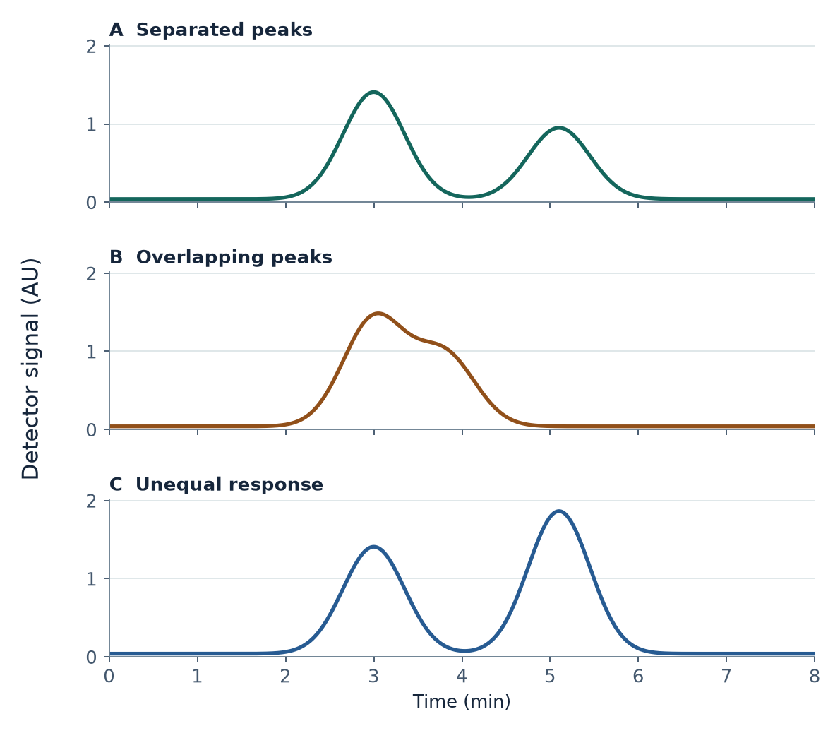
Three files contain 801 points each, from 0.00 to 8.00 min in 0.01 min steps. The UTF-8 CSVs use comma delimiters and decimal points. Columns time_min and detector_signal_au contain time and the combined signal, including a constant 0.040 AU baseline. No component columns are supplied.
Practice: plot, resolve, integrate
- Plot A, B and C on the same axes. Compare the observed maxima with the known model centers in the worksheet.
- Subtract the 0.040 AU baseline. Integrate by the trapezoid rule and compare vertical splits of the combined signal.
- Calculate resolution from the model widths. Correct component area ratios for known response factors and state why integration cannot fully separate coeluting signals.
Model and assumptions
Two ideal Gaussian signals and a constant baseline generate each trace. There is no noise, drift or tailing. Case A has separated peaks and equal detector response. Case B moves the centers closer together. Case C keeps the reference separation and increases the response of the later component.
Worked answers
The original instructor guide supplies the full parameter table, numerical integration procedure and worked answers. Use the documented limits and split positions when reproducing those results. A visually clean maximum does not prove that only one component is present.
Teaching notes
Ask learners to inspect combined signals before seeing the component curves. Keep axis ranges fixed, check units and require an interpretation alongside the calculation. The models represent no measured sample.
Provenance and reuse
Synthetic teaching model — no laboratory measurement.
Original teaching text and synthetic data: CC BY 4.0. Third-party references retain their own terms.
Creative Commons Attribution 4.0 International
IUPAC: Nomenclature for Chromatography, §§ 3.3.06–3.3.07, 3.10.01